Estimating the number of fish that return to spawn using capture-recapture methods.
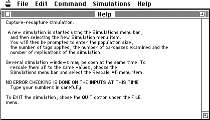
First, download the Xlisp-stat module, let it start, and return to this page. If the downloading was successful, your screen
should appear similar to:

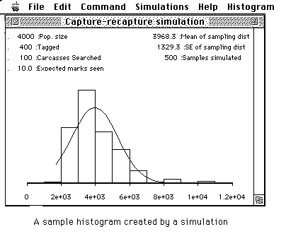
The computer simulation allows you specify the population size, the number tagged, the number of carcasses searched and the number of replications to perform. It then draws a histogram of the estimates from the replications, fits a 'normal curve' to the histogram, and computes the average and standard deviation of the estimates.
There is one slight complication. Looking at the formula for the estimate of ![]() you see that
m2 appears in the denominator. If m2 has the value of zero, the estimator is undefined. Consequently, a revised estimator is often used to avoid this problem:
you see that
m2 appears in the denominator. If m2 has the value of zero, the estimator is undefined. Consequently, a revised estimator is often used to avoid this problem:
        (n1+1)(n2+1)
   * = ----------- - 1
          (m2+1)
This is what is used in the computer simulation.
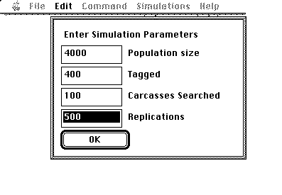
Lets repeat our simulation using 500 replications. A sampling experiment is started by clicking on the "Simulation" menu bar in the Xlisp-stat module and selecting the "New Simulation" menu item (you will have to change focus to switch to the module). Then you fill in the various terms.
For example, to simulate the sampling bowl experiment, fill in the following values on the computer simulation and then click on the OK button to launch the simulation:

After a few seconds a histogram will be shown similar to the following:

You may resize the histogram and move it about on the screen. Try it and then return to this screen.
Are the results similar to those that you obtained in your hand simulation? Move the histogram window to the bottom of your screen.
Most people would agree that estimates from larger samples are "better." Repeat the above computer experiment using more carcasses searched, say 200 (but keeping all the other values the same), by selecting the "Simulation" menu bar again. After both simulations have been run, your screen would look similar to this example.
Compare the histogram of the estimates for carcass samples of size 200 with the histogram for a carcass samples of size 100. Describe in what ways estimates from larger samples are "better." [In order to make a better comparison, make the scales for all the windows the same. Choose the "Simulation" menu bar, and select the "Rescale All" menu item.]
Find the ratio of the standard error using a carcass sample of size 200 to a carcass sample of size 100. What happens to the standard error when the carcass sample size is doubled? What do you think the standard error will be with a carcass sample size of 400? [You can verify your results using the simulator].
You saw above that increasing the numbers of carcasses examined (while keeping the number tagged the same) lead to a smaller sampling variation. It turns out that the number of tags recovered is what is important and that various combinations of the number of tags applied and the number of carcasses examined lead to essentially the same sampling distribution.
The expected number of tags recovered can be computed as:
                                                   n1
   E[m2] = fraction marked x carcasses searched =  -- n2
                                                   N
For example, the first computer simulation had N=4,000, n1=400 and n2
=100 which gives:
             400
   E[m2] = ----- x 100 = 10.
           4,000
The second computer simulation had N=4,000, n1=400, and n2 increased to 200.
This gives:
             400
   E[m2] = ----- x 200 = 20
           4,000
and we saw that the sampling distribution in the latter case was less variable
(i.e. had a smaller standard error) than the first simulation.
What is the expected value of m2 (the number of tags seen again) if the population has 4000 fish, 400 tags are applied and 100 carcasses are examined? How do you think the standard error will compare to the two previous simulations?
What is the expected number of tags returned if the population has 4000 fish, 800 tags are applied and 50 carcasses examined? How will its standard error compare to the two previous cases?
You can verify your computations using the simulation program. Notice that the shape of the sampling distribution is similar as long as the expected value of m2 is the same.
In more advanced classes, you will see that the standard error for a Petersen experiment can be approximated by
Finally, use the above formula to estimate the standard error for the Chilko River estimate that you looked at earlier. Using the empirical rule, find an interval for the plausible size of the spawning population.