Jim Albert
Bowling Green State University
Journal of Statistics Education v.3, n.3 (1995)
Copyright (c) 1995 by Jim Albert, all rights reserved. This text may be freely shared among individuals, but it may not be republished in any medium without express written consent from the author and advance notification of the editor.
Key Words: Baseball; Bayes' rule; Conditional probability; Prediction; Prior distribution.
Teaching elementary statistical inference from a traditional viewpoint can be hard, due to the difficulty in teaching sampling distributions and the correct interpretation of statistical confidence. Bayesian methods have the attractive feature that statistical conclusions can be stated using the language of subjective probability. Simple methods of teaching Bayes' rule are described, and these methods are illustrated for inference and prediction problems for one and two proportions. We discuss the advantages and disadvantages of traditional and Bayesian approaches in teaching inference and give texts that provide examples and software for implementing Bayesian methods in an elementary class.
1 Consider the teaching of a one semester introductory statistics course for liberal arts majors. To introduce statistical inference to this audience, many statistical educators believe that it is not necessary to teach particular methods, such as a t-test or analysis of variance. Rather the emphasis should be on teaching general inferential concepts. One important concept is the distinction between populations and their summaries (parameters) and samples and their summaries (statistics). A second significant idea in inference is the meaning of statistical confidence, in particular, the interpretation of a 95% confidence interval. The student should understand the role of sample size; generally, more data from a random sample gives one more information about a parameter. Another basic notion is the dependence of statistical conclusions on assumptions about the sampling process and the probability model.
2 The traditional approach to teach the above inferential concepts is based on the relative frequency notion of probability. Although this approach is implemented in practically all elementary statistics textbooks, it can be difficult to teach. In particular, it can be hard for students to distinguish a parameter, such as a population proportion p, from the proportion statistic \hat{p} that is computed from a sample. The idea of a sampling distribution is often mysterious to students. There are many concepts included in a discussion of a sampling distribution, such as the notion of taking a random sample, computing a statistic from the sample, and then repeating the process many times to understand the repeated sampling behavior of the statistic. In addition, it can be difficult to communicate the correct interpretation of statistical confidence statements. If a student computes a 95% confidence interval from a particular sample, he or she may think that this particular interval contains the parameter of interest with a high probability. The student has to be corrected -- in classical inference, one is confident only in the coverage probability of the random interval. Likewise, a p-value can be misinterpreted as the probability of the null hypothesis instead of the probability of observing a sample outcome at least as extreme as the one observed. This error is easy to make since the notion of a p-value is not intuitive. If data are collected, one is interested in the degree of evidence that is contained in the observed data in support of the null hypothesis. Why should one be concerned with the probability of sample outcomes that are more extreme than the one observed?
3 Consider the teaching of the above inferential concepts by a Bayesian approach. In inference, one is uncertain about the values of population parameters, and one gains additional information about the parameters from observed data. In Bayesian inference, the uncertainty about parameters is expressed using subjective probability, and Bayes' rule is the mechanism for updating one's subjective knowledge from data.
4 One difficulty in teaching classical statistics is communicating the correct interpretation of statistical "confidence." Bayesian confidence statements can be more familiar to students since one's knowledge about parameters is described using the language of probability. Given observed data, one can talk about the probability that a fixed interval contains a population parameter, or the probability that a statistical hypothesis is true. So a 95% Bayesian interval estimate for a proportion p is an interval that contains p with probability .95. If one has a coin with probability of heads p, then one can consider the probability of the hypothesis that the coin is fair (p = .5).
5 A second attractive feature of Bayesian inference, from the viewpoint of teaching, is that inferences are made conditional on the observed data. In classical statistics, one must think about the possibilities of data sets distinct from that one that is actually observed. In Bayesian inference, the only data set relevant for drawing conclusions is the data set that you see.
6 Despite the above benefits, the Bayesian approach in teaching inference requires the teaching of new material that may be excluded from a traditional statistics class. Specifically, the students need to understand the subjective interpretation of probability and conditional probability. Bayes' rule has to be taught as the method of changing one's conditional probabilities given new information.
7 How does one teach Bayes' rule? Since parameter spaces for a proportion or mean are continuous-valued, it might seem on the surface that one has to consider continuous-valued prior distributions for a parameter. Summarizing the posterior density in this case may involve analytical or numerical integration which can present computational problems. However, the basic tenets of Bayesian inference can be communicated in the simpler discrete setting where there is a small set of parameter values of interest.
8 The aim of this article is to illustrate how Bayes' rule applied to a discrete set of parameter values can be used to teach inference and prediction about one and two proportions. Section 2 presents Bayes' rule in a simple tabular form that is relevant for learning about a proportion p. One has a set of plausible values of the proportion and one updates one's knowledge about the values of p after observing the results of a binomial experiment. The law of total probabilities provides a simple mechanism for predicting the results of a future binomial experiment. The examples in Section 3 provide illustrations of Bayesian prediction and inference for problems involving one and two proportions. In Section 3.1, the problem is to predict the number of home runs Matt Williams would have hit if the 1994 baseball season had not ended prematurely due to the strike. We illustrate constructing a prior distribution for Williams' home run proportion for three hypothetical fans and seeing the effect of one's opinion about Williams' home run ability on the prediction of interest. In Section 3.2, we compare two proportions from a medical trial on the basis of two independent samples. In Section 4, we describe our experiences in teaching elementary statistics from a Bayesian viewpoint, and in Section 5 we summarize the advantages and disadvantages of teaching basic inference using traditional and Bayesian perspectives.
9 Bayes' rule is often presented in a chapter that introduces probability theory. However, it usually is not introduced from a statistical perspective. Suppose one is interested in learning about a proportion p. The actual value of p is unknown, but suppose that one can construct a set of plausible values for p, which we denote by p_1,..., p_k. If the student cannot think of a set of plausible values, then an equally spaced grid of proportion values from 0 to 1 will suffice for many problems.
10 Next, one assigns probabilities to the different values of p that reflect one's belief about which values are more or less likely to be true. Let the proportion values p_1,..., p_k have respective probabilities P(p_1),..., P(p_k). It is generally difficult for students to make these probability assignments, since they have had little practice in thinking about the sizes of probabilities. However, a student may be able to make a "best guess" at p and then construct a symmetric distribution about this most likely value. One could place equal probabilities on the k values for p, indicating that it is difficult to make judgments between them. (We will illustrate constructing a prior distribution in Section 3.1.) The important aspect of this process is that the student has to think about the interpretation of the proportion p for the particular application.
11 To learn more about the value of p, a binomial experiment is performed; suppose that you observe s successes and f failures. By Bayes' rule, the updated probability of the value p is proportional to the product
P(p) x P(s successes, f failures | p), (1)
where P(s successes, f failures | p) = p^s(1-p)^f is the likelihood or the probability of observing a particular sequence of successes and failures (with total number of successes and failures s and f) if the proportion value is equal to p. To compute the set of updated probabilities for all values of p, one computes the product above for all values, computes the sum of these products, and then divides each individual product by the sum to obtain probabilities.
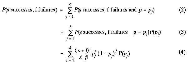
12 A second type of inference is to predict the results of a future binomial experiment. Suppose, as above, there are k possible values for the proportion, p_1,..., p_k, with respective probabilities P(p_1),..., P(p_k). You are interested in the probability of observing s successes in a future binomial experiment of s + f trials. Using the law of total probabilities,
In the above expression, the probabilities {P(p_j)} can represent prior probabilities before any data have been observed or posterior probabilities after observing data. The probability of s successes for a given value of p is given by the binomial formula.
13 The above formula can be used to compute the predictive probability for any values of s and f. The set of predictive probabilities {P(s successes, f failures)} can be used in a number of ways. By computing predictive probabilities for different sets of prior distributions, the student can assess his/her choice of prior. It may be easier to think about the number of successes in a future experiment of a given sample size than to directly think about the population proportion. Also, one can see what has been learned from the observed data by comparing the predictive probabilities based on the prior distribution with the predictive probabilities based on the posterior distribution.
14 Bayes' rule in this discrete case is illustrated in the tabular format shown in Table 1. In this example, a grid of equally spaced values of the proportion p is used. The columns of the table give the values of the proportion, the prior probabilities, the likelihoods, the products, and the posterior probabilities. The sum of the products, indicated by `SUM' in the table, is the predictive probability (based on the prior probabilities) of a particular sequence of s successes and f failures.
 Model  Prior    Likelihood          Product               Posterior
   0     P(0)   (0)^s(1-0)^f     P(0)(0)^s(1-0)^f     P(0)(0)^s(1-0)^f/SUM
   .1   P(.1)  (.1)^s(1-.1)^f  P(.1)(.1)^s(1-.1)^f  P(.1)(.1)^s(1-.1)^f/SUM
   .2   P(.2)  (.2)^s(1-.2)^f  P(.2)(.2)^s(1-.2)^f  P(.2)(.2)^s(1-.2)^f/SUM
   .3   P(.3)  (.3)^s(1-.3)^f  P(.3)(.3)^s(1-.3)^f  P(.3)(.3)^s(1-.3)^f/SUM
   .4   P(.4)  (.4)^s(1-.4)^f  P(.4)(.4)^s(1-.4)^f  P(.4)(.4)^s(1-.4)^f/SUM
   .5   P(.5)  (.5)^s(1-.5)^f  P(.5)(.5)^s(1-.5)^f  P(.5)(.5)^s(1-.5)^f/SUM
   .6   P(.6)  (.6)^s(1-.6)^f  P(.6)(.6)^s(1-.6)^f  P(.6)(.6)^s(1-.6)^f/SUM
   .7   P(.7)  (.7)^s(1-.7)^f  P(.7)(.7)^s(1-.7)^f  P(.7)(.7)^s(1-.7)^f/SUM
   .8   P(.8)  (.8)^s(1-.8)^f  P(.8)(.8)^s(1-.8)^f  P(.8)(.8)^s(1-.8)^f/SUM
   .9   P(.9)  (.9)^s(1-.9)^f  P(.9)(.9)^s(1-.9)^f  P(.9)(.9)^s(1-.9)^f/SUM
   1     P(1)   (1)^s(1-1)^f     P(1)(1)^s(1-1)^f     P(1)(1)^s(1-1)^f/SUM
                                       SUM                     1
Table 1: Computation of posterior probabilities for a proportion with a discrete prior on a grid of values from 0 to 1 and an observed sample of s successes and f failures.
15 The 1994 baseball season was particularly exciting, since there were a relatively large number of runs scored, and particular players had great hitting seasons. Some players appeared to have reasonable chances of exceeding the single season record of 61 home runs, and one player was close to having a .400 batting average. Unfortunately, the baseball season ended due to a strike on August 11, and fans were left to wonder what would have happened to particular batting records if a full 162 game season had been played.
16 In particular, let's consider Matt Williams who, on August 11, had hit 43 home runs in his first 445 at-bats. If the baseball strike had not occurred, assume that Matt Williams would not be injured and would have 199 additional at-bats during the remainder of the season. (This number of at-bats is an estimated number of at-bats used by Cramer and Dewan (1995) in their simulation of the 1994 season.) Did he have a reasonable chance of hitting more than a total of 61 home runs and setting the home run record? In other words, was it likely that Williams would hit at least 19 home runs in his final 199 at-bats?
17 The answer to this question depends on one's opinion about Williams' home run hitting ability during the last part of the season. One could assume that his rate of hitting home runs would remain similar to the rate displayed during the first part of the season, or one could regard Williams as unusually "hot" during the first 445 at-bats and expect him to cool down during the remainder of the season.
18 Suppose that one views individual at-bats during the last part of the season as independent Bernoulli trials where p is the probability of Williams hitting a home run during a single plate appearance. What is the interpretation of the home run rate parameter p? This is the proportion of home runs of Williams if he was allowed to take a hypothetical large number of at-bats under identical conditions during this last part of the season. In teaching, it is important to distinguish this probability value from the sample proportion \hat{p} of home runs that Williams might hit during his final 199 at-bats. Also, the value of p represents Williams' home run ability only during this last part of the season. It is very possible that Williams' probability of hitting a home run changes during the course of a season. It is also possible that Williams' home run hitting ability changes over the course of his career. His home run hitting probability during the end of the 1994 season could be very different than his chances of hitting home runs during previous years.
19 After one understands the meaning of the Bernoulli parameter p, one constructs a probability distribution on a set of plausible values for p that reflects one's beliefs about Williams' home run ability during the remainder of the 1994 season. Since one's opinion about Williams' ability can vary, let us consider the beliefs of three hypothetical baseball fans, Allan, Bob, and Sally. In the following, we discuss the opinions of these three fans about Williams' home run ability, and describe how one can construct a probability distribution for each fan that matches the individual opinions.
20 The first fan, Allan, believes that Williams' home run ability for the remainder of the 1994 season is best measured by his performance during the first part of the 1994 season. In fact, he thinks that Williams' probability of hitting a home run, p, would be the same over the entire season. In addition, he believes that Williams' home run performance in previous years is irrelevant for learning about his performance during 1994. In other words, Allan believes that Williams' home run probability in 1993 and earlier years is different from his 1994 home run probability. This could be due to a new batting swing or stance or perhaps to some extra strength training during the off-season.
21 Since Allan believes that Williams' probability p remains constant over the entire 1994 season, he will use the batter's home run data in the observed first part of the season to construct his probability distribution. Allan initially knows very little about the value of p, so he considers a large set of possible home run rates {.01, .02, .03,..., .20} and assigns each value in this set the same probability. Using the method described in Section 2, he updates his probabilities with the 1994 data -- s = 45 successes and f = 402 failures, where we define a success as hitting a home run. The revised probabilities for Allan are shown in Table 2.
    p     .01  .02  .03  .04  .05  .06  .07  .08  .09  .10  .11  .12  .13  .14
 Allan's   0    0    0    0    0    0   .03  .13  .25  .28  .19  .08  .03  .01
  Bob's    0    0    0   .14  .14  .14  .14  .14  .14  .14   0    0    0    0
 Sally's  .06  .06  .06  .12  .19  .19  .12  .06  .06  .06   0    0    0    0
Table 2: Three prior distributions for Matt Williams' home run rate.
22 The second fan, Bob, has a different opinion about Williams' home run ability for the remainder of the 1994 season. He thinks that Williams' batting performance in his previous major league seasons is relevant for learning about p. So Bob looks at Williams' home run statistics for the previous five seasons. Table 3 displays the number of at-bats, the number of home runs, and his observed home run rate for these earlier seasons. For each season, one can also learn about the corresponding season home run probability by the method of Section 2. One can assume a priori that the home run probability is uniform over the grid of values {.01, .02,..., .20}, and obtain a posterior distribution for the probability using the observed data from the season. In Table 3, the column 'TRUE RATES' lists values for the season home run probability that received a posterior probability of at least .01. In 1989, for example, Williams hit 18 home runs in 292 at-bats for an observed home run rate of .062. This season hitting data is consistent with home run probabilities of .04, .05, .06, .07, .08, and .09.
      YEAR  HOME RUNS  AT-BATS  OBS. RATE               TRUE RATES
      1989      18       292       .062       {.04, .05, .06, .07, .08, .09}
      1990      33       617       .053         {.04, .05, .06, .07, .08}
      1991      34       589       .058         {.04, .05, .06, .07, .08 }
      1992      20       529       .038         {.02, .03, .04, .05, .06 }
      1993      38       579       .066        { .05, .06, .07, .08, .09 }
      1994      43       445       .097    {.07, .08, .09, .10, .11, .12, .13}
Table 3: Home run statistics for Matt Williams for his years in the major league.
23 After looking at the calculations summarized in Table 3, Bob has some idea about Williams' home run probabilities for the years 1989 - 1993 and the first part of the 1994 season. He is reluctant to pool all of the home run data from previous years, since he believes that Williams' home run ability has changed from 1989 through 1994. But he thinks that the value of the home run probability p for the remainder of the 1994 season is among the plausible home run probabilities from previous seasons. After some reflection, he thinks that p is contained in the set {.04, .05,..., .10}. He notes that Williams' home run probability in 1992 could have been as low as .02, but he thinks that Williams will be hitting better in the remainder of 1994 than he hit in 1992. It is possible, from the observed data in 1994, that Williams' home run probability could be as high as .13. But Bob feels that this is too big an improvement from the probability values of previous seasons, so he places an upper bound of .10 on Williams' home run probability for the end of 1994. It is hard for Bob to prefer particular values of p, so he decides to assign each value in the set {.04, .05,..., .10} the same prior probability.
24 Sally's opinions about Williams differ from those of the previous two fans. She has been particularly impressed with the home runs that Williams has hit in the first part of 1994. However, she thinks that Williams has been "hot" during the first part of the season and thinks it would be difficult for him to continue to hit home runs at this hot rate for the remainder of the season. Also, there will be additional pressure placed on Williams during the remainder of the season. The single season home run record of 61 was set over 30 years ago, and Williams will receive extensive media coverage if he gets close to the record. This extra media pressure could have an adverse effect on Williams' hitting ability during this time. (An alternative explanation for this belief is the well-known regression effect. In this setting, the regression effect is the phenomena that players who have extreme batting performances in the first half of a season will tend to have more average performances during the second half of the season.)
25 How does Sally construct her prior distribution for p? From looking at Williams' home run record from previous seasons, she thinks that a plausible set of values for p is from .01 to .10. She feels that Williams will cool down from the .097 rate that he displayed in the first part of the 1994 season. She places the largest probabilities on the values of .05 and .06 which are more consistent with Williams' performance during previous years. Although .05 and .06 are the most probable values of p, Sally thinks that there is a small chance that Williams will rise to the occasion and break the home run record. Also, there is a small chance that Williams will display a significant slump and hit very few home runs during the remainder of the season. So she assigns probabilities on p that slowly decrease as one moves away from the most probable values. The extreme home run probabilities of .01 and .10 receive prior probabilities of .06.
26 What is the implication of these different beliefs about Williams' home run rate p on the predictions that he will break the home run record? Using the basic formula of Section 2, one can compute the predictive probabilities of the number of home runs y for each of the three fans. The plots of these probability distributions are shown in Figure 1. The first thing to notice is that there is substantive variability for each prior in the number of home runs Williams will hit in the remainder of the season. For example, if Allan's prior is used, then Williams could hit anywhere between 10 and 30 additional home runs. Second, these three predictive distributions vary significantly with respect to location and spread, indicating that one's prior probabilities about Williams' home run rate can have a large impact on one's prediction of his performance during the remainder of the season.
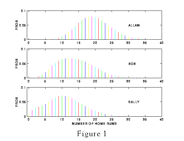 Figure 1 (6.9K gif)
Figure 1. Predictive Probabilities of Number of Home Runs for the Remainder of the Season for Allan, Bob, and Sally.
27 Specifically, we are interested in computing the probability that Williams will break the home run record, which is the probability that the number of home runs, y, is 19 or greater. This probability is easily computed from one's predictive distribution -- one sums the predictive probabilities for all values of y equal to 19 or greater. For the three prior distributions corresponding to Allan, Bob, and Sally, this probability is given by .571, .205, and .099, respectively. These three fans have very different probabilities that Williams would have broken the record.
28 A baseball fan who looks at the above calculations may wonder who to believe; is it possible to reconcile the above analyses? The answer is no. This example illustrates the sensitivity of statistical conclusions to assumptions. To predict Matt Williams' home run performance, one must make some assumptions about how his future home run hitting ability (measured by the probability p) is related to what he displayed in previous seasons and the first part of the 1994 season. Since these assumptions critically affect the final conclusion, it makes one think about one's assumptions more carefully. Personally, although I was impressed with Williams' home run performance in 1994, I view the season home run record as a very difficult hurdle to overcome, so I would give the record breaking event {y \ge 19} a relatively small probability. The implication of this belief is that I think that Williams' home run probability p for the remainder of the season would be small, and I would assign probabilities similar to those assigned by Bob or Sally. Likewise, another baseball fan would have to think about her prior beliefs about Williams' home run ability to form her personal prediction of Williams' breaking the home run record.
29 The discrete approach to teaching Bayesian inference is also useful in the comparison of two unknown parameters. To illustrate the use of this approach, we analyze data from the famous ECMO study. (A discussion of this study is given in Ware 1989. These data are presented in an exercise in Berry 1995.) Researchers at Harvard were interested in comparing two treatments for newborn babies suffering from severe respiratory failure. The two treatments were a conventional therapy CMT and a radical experimental therapy ECMO. Let p_C and p_E denote the population proportions of infants with this respiratory condition that would survive under the treatments CMT and ECMO, respectively.
30 Before the study was conducted, the Harvard researchers had some prior information about the sizes of the two proportions. Based on historical experience, it was believed that approximately 20% of infants with this condition survive under conventional therapy. In addition, an earlier study at the University of Michigan provided encouraging information about the effectiveness of the ECMO treatment. These researchers used a randomization procedure that assigned a therapy to a patient based on its success on previous patients. In this Michigan study, all 11 infants assigned to the ECMO therapy survived, and the one infant assigned to CMT therapy died. There was some concern about the usefulness of this study since only one infant was given the conventional therapy.
31 In the Harvard study, a two-phase study was performed. In the first phase, 6 of the 10 infants assigned to the CMT treatment survived, and all 9 infants assigned to ECMO survived. Since ECMO was the more effective treatment in the first phase, the second phase of the study treated 20 new patients with ECMO, and 19 infants survived. Combining the results from the two phases, of 10 infants treated with CMT, 6 survived, and of 29 infants treated with ECMO, 28 survived.
32 In this setting, two types of inference will be considered. First, one may wish to test the hypothesis that the two proportions are equal. A Bayesian test of equal proportions is found by first constructing a prior distribution that assigns the hypothesis of equality a fixed probability and then computing the posterior probability of this hypothesis. The second type of inference is estimation. Suppose that the Harvard doctors are interested in estimating the benefit of the ECMO treatment measured by the difference in proportions d = p_E - p_C. In this estimation problem, we will illustrate the construction of a subjective probability distribution to reflect prior knowledge of the effectiveness of the two treatments.
33 The discrete approach of Section 2 for one proportion can be generalized in a straightforward manner to this example. First, consider the testing application. We set up a grid of plausible values for p_C and p_E. Assume little is known a priori about the survival proportions, so a grid of 11 values is constructed for each proportion equally spaced between 0 and 1. The next step is to assign probabilities for each pair of proportion values (p_C, p_E). The researchers wish to test the hypothesis that the two treatments are equally effective and the proportions of survival are equal (p_C = p_E). Moreover, suppose that they believe a priori that the probability that the proportions are equal is .5. (They do not trust the information provided by the historical data and the earlier studies.) A prior distribution that models this information is constructed by slightly modifying the uniform distribution. We assign to each proportion pair along the diagonal the same probability, and each pair off the diagonal the same probability such that the total probabilities of the diagonal section and the off-diagonal sections are both one half. The resulting prior is displayed in Table 4.
      p_C\p_E   0  .1  .2  .3  .4  .5  .6  .7  .8  .9   1
         0     45   5   5   5   5   5   5   5   5   5   5
        .1      5  45   5   5   5   5   5   5   5   5   5
        .2      5   5  45   5   5   5   5   5   5   5   5
        .3      5   5   5  45   5   5   5   5   5   5   5
        .4      5   5   5   5  45   5   5   5   5   5   5
        .5      5   5   5   5   5  45   5   5   5   5   5
        .6      5   5   5   5   5   5  45   5   5   5   5
        .7      5   5   5   5   5   5   5  45   5   5   5
        .8      5   5   5   5   5   5   5   5  45   5   5
        .9      5   5   5   5   5   5   5   5   5  45   5
         1      5   5   5   5   5   5   5   5   5   5  45
Table 4: Prior distribution of two proportions from the ECMO study. Each entry in the table represents 1000 times the prior probability.
34 Once this prior is constructed, the implementation of Bayes' rule is straightforward and follows the same recipe as in the one proportion case. For each proportion pair (p_C, p_E), we compute the likelihood or the probability of the above sample result (6 out of 10 survived for CMT, 28 out of 29 survived for ECMO) for a given set of proportions:
L(p_C, p_E) = (p_C)^6 (1-p_C)^4 (p_E)^{28} (1-p_E)^1Next, the prior values are multiplied by the likelihood values, and the values are normalized to make probabilities; the resulting posterior probabilities for (p_C, p_E) are shown in Table 5.
       p_C\p_E  0  .1  .2  .3  .4  .5  .6  .7   .8   .9   1
         0      0   0   0   0   0   0   0   0    0    0   0
        .1      0   0   0   0   0   0   0   0    0    0   0
        .2      0   0   0   0   0   0   0   0    0    5   0
        .3      0   0   0   0   0   0   0   0    2   32   0
        .4      0   0   0   0   0   0   0   0    7   98   0
        .5      0   0   0   0   0   0   0   0   13  179   0
        .6      0   0   0   0   0   0   0   1   16  220   0
        .7      0   0   0   0   0   0   0   5   13  176   0
        .8      0   0   0   0   0   0   0   0   57   77   0
        .9      0   0   0   0   0   0   0   0    1   98   0
         1      0   0   0   0   0   0   0   0    0    0   0
Table 5: Posterior distribution of two proportions from the ECMO study. Each entry in the table represents 1000 times the posterior probability.
35 Many things can be learned from this matrix of probabilities. Since many more babies received the ECMO treatment, one has much more information about the corresponding population proportion value. From the table, we see that most of the probability for p_E is concentrated near .9, while the probabilities for p_C are spread out from .3 to .9. Is it likely that the proportions are equal? A priori the probability of the diagonal cells was equal to .5. From summing the posterior probabilities for the diagonals, we see that the posterior probability of equality has dropped to .16. Thus there is some evidence from the data that the proportions are unequal.
36 Now suppose that the inference of interest is estimating the benefit of the ECMO treatment, and the Harvard researchers wish to use the information that is available from previous studies. Suppose, as above, an 11 by 11 grid of proportion values is used. It is certainly more difficult to specify a joint probability distribution for the two proportions when one has significant prior information. However, some assumptions can be made to simplify this probability assessment. In the following, we will construct a prior distribution for each proportion based on the researchers' knowledge and assume that the two distributions are independent to construct a joint distribution.
37 First consider the proportion of infants p_C that survive under the conventional treatment. The Harvard team knows that the conventional therapy has an approximate 20% survival rate. Specifically, in one particular historical dataset, only 2 of 13 patients survived. Since the doctors are not sure if the historical patients are exchangeable with the patients in their study, they wish to downweight this information. The resulting prior distribution for p_C is displayed in Table 6. This distribution reflects the belief that p_C is most likely to be in the .1 - .3 range. The Harvard researchers know less about the ECMO survival proportion p_E, thus the distribution for p_E will be more diffuse than the distribution for p_C. However, based on the Michigan study, the researchers believe that it is possible that ECMO is a much better treatment. The prior distribution for p_E gives significant mass to proportion values between .1 and .6.
            p       0   .1   .2   .3   .4   .5   .6   .7  .8   .9   1
       Prior - CMT  0  .28  .30  .21  .12   .6   .3   0    0    0   0
      Prior - ECMO  0  .18  .18  .17  .14  .12  .09  .06  .04  .02  0
Table 6: Marginal prior distributions of the survival probabilities using the CMT and ECMO treatments.
38 By the independence assumption, the joint probability distribution is found by multiplying the two marginal distributions given in Table 6. From this distribution, one can compute that the probability that p_E > p_C is .576 and the probability that p_E < p_C is .257. This prior expects ECMO to have a significantly higher survival rate.
39 After the Harvard study is completed, the prior probabilities for the proportions are updated in the same manner as the testing situation. A grid of posterior probabilities is obtained; from this grid, one can compute the posterior distribution for the difference in proportions which is given in Table 7. Note that approximately 94% of the posterior probability is contained in the values d = .3, .4, .5, .6. Thus one is 94% confident that the ECMO treatment provides a 30-60% improvement in the survival rate over conventional therapy.
40 To see the effect of the informative prior on the above conclusions, one can reanalyze these data using a uniform prior distribution on the grid of values of the two proportions. Table 7 also gives the posterior distribution for the improvement in survival rates using this uniform prior. One sees from this table that most of the posterior probability is concentrated on values of the improvement from .1 to .5. The two posterior distributions have similar locations and spreads. Since the Harvard researchers had some prior information about the superiority of the ECMO therapy, they can give a higher estimate of the improvement in survival rates.
Prior     p_E-p_C   -.1    0    .1    .2    .3    .4    .5    .6    .7    .8  .9
Subjective  PROB     0     0   .001  .025  .192  .291  .295  .162  .033  .001  0
Uniform     PROB   .001  .019  .106  .224  .272  .218  .117  .038  .006   0    0
Table 7: Posterior distribution of the improvement of survival probability using the ECMO treatment using subjective and uniform priors.
41 The Bayesian methods described in Sections 2 and 3 were implemented in a three-hour elementary statistics class. The course was designed as a one-semester course for non-mathematics majors. It is expected that this will be the only course in statistics for the student. The general goal is to introduce the student to the use of statistical reasoning in the real world. Since the students do not have to learn particular statistical methods such as a t-test, the instructor has some freedom of choice on the methods that are presented.
42 The class was taught completely from a Bayesian perspective using Berry (1995). The topics covered were standard: data analysis, collecting data, probability, inference about proportions and means, and simple linear regression. Bayes' rule was used throughout to make inferences about parameters. There was no discussion of classical inference including sampling distributions and the relative frequency interpretation of interval estimates and tests.
43 For a particular problem, say, learning about a single proportion, inference was introduced by means of the discrete Bayes approach described in Section 2. After some experience with the use of a discrete prior density with a small number of proportion values, a large number of proportion values was used to motivate the use of continuous beta prior distributions. Discrete priors were also used to motivate inference about two proportions and a population mean from a normal distribution.
44 The class met three times a week -- two days of lectures and one day in a computer lab. In the lab, the students were given a worksheet with a number of inferential problems. In a typical problem, students were asked to formulate their prior distribution for the unknown parameters; data were given, and the posterior calculations were performed using Minitab. In one lab, the students were interested in learning about the average number of brown candies in a snack size bag of M&M;'s. They were asked questions about their prior opinion, and a Minitab program was used to fit a normal density to this opinion. Then they counted the number of brown candies in a bag and updated their opinion on the computer using a second Minitab program.
45 Another important component of the class was a project including a statistical analysis. The class was divided into small groups, and each group formulated a question of interest. One group was interested whether female students on a diet on campus were more likely to exercise than female students not on a diet. They wrote down their initial impressions and constructed a prior for the proportions of exercisers and non-exercisers on a diet. Then they took a random sample of students by a telephone survey, updated their prior probabilities, and summarized what they learned.
46 This project may have been the most beneficial part of the class. The students learned the scientific method and found the course more relevant since they were working on problems that interested them. The construction of the prior was helpful for the students in describing (before sampling) what they hoped to learn from the survey. It is interesting to note that the students tended to be somewhat conservative in the specification of their prior distributions, and the posteriors tended to be dominated by the observed data.
47 This article has demonstrated the use of Bayesian inference with discrete priors to teach binomial inference and prediction. Although this article has focused on proportion problems, this approach can be used for a large variety of inference problems. Berry (1995) introduces elementary statistical inference completely from a Bayesian perspective and uses the discrete model approach for performing inferences about one and two proportions and means. In Albert (1996), the use of discrete models and Bayesian updating is illustrated for inference problems for normal, exponential, Poisson, hypergeometric, and uniform distributions.
48 In comparing Bayesian and classical approaches in teaching, it is important to remember the basic goals of our first statistics class. Many statistics classes are designed to serve particular disciplines, such as biology, business, or education. In these classes, one goal may be to teach particular methods and corresponding classical interpretations of these methods so that students will be able to understand statistical reports in their discipline. For these classes, the traditional approach may be necessary.
49 Other elementary statistics classes are not designed for a particular discipline. The goal of these classes is to introduce the students to the use of statistics in learning by means of the scientific method. This article suggests that a Bayesian viewpoint may be preferable to a traditional viewpoint in communicating basic tenets of statistical inference for this liberal-arts-oriented class. The point is not that the traditional approach to inference has fundamental flaws. (The author prefers the Bayesian approach, but the reasons for this preference are best presented in a more advanced statistics class.) Rather, the instructor may have more success in teaching concepts such as confidence, the role of sample size, and the distinctions between populations and samples using a Bayesian viewpoint.
50 Table 8 summarizes the advantages and disadvantages of Bayesian and traditional viewpoints in teaching. Many of these points have already been discussed in this paper. The main advantage of the traditional approach is its familiarity. The classical methods are well-known, and the frequency interpretation is the common one for interval estimates and tests of hypotheses. Traditional methods are generally viewed as objective, which is desirable.
                     TRADITIONAL                   BAYES

      Advantages     familiar procedures           natural interpretation
                     used in industry              of statistical
                     and software                  confidence

                     automatic, easy to use        confidence statements
                     procedures                    are conditional on
                                                   observed data

                     procedures are "objective"    focuses on interpretation
                                                   of parameters

                                                   Bayes' rule provides an
                                                   automatic method of
                                                   updating probabilities

      Disadvantages  teaching sampling             teaching conditional
                     distributions                 probability

                     teaching "repeated            teaching subjective
                     sampling" interpretation      probability
                     of confidence

                     focus on methods              teaching specification
                     rather than concepts          of prior distributions

                                                   teaching Bayes' rule
Table 8: Advantages and disadvantages of teaching inference using traditional and Bayesian methods.
51 However, the traditional approach to teaching has disadvantages; here a disadvantage can refer to an idea that is difficult to communicate. As mentioned in Section 1, this approach requires the discussion of the concept of sampling distributions. Since this is a hard idea, it is difficult to communicate the correct interpretation of confidence. The table also criticizes the traditional approach for its focus on inferential methods rather than concepts. This may be better stated as a criticism of the current statistics textbooks and teachers. But the emphasis on methods may be a consequence of the difficulty in teaching the basic concept of confidence based on repeated sampling -- it is certainly easier to teach methods than ideas.
52 Table 8 also summarizes the main advantages and disadvantages of the Bayesian approach. One key advantage is that it focuses attention on the population parameter. To construct a discrete-type prior distribution for a proportion p, the students are motivated to understand what p really means in the particular example. In the baseball example of Section 3.1 there can be confusion about the interpretation of Williams' home run rate, and the discussion of constructing a prior can help in understanding this key parameter. Unfortunately, in traditional teaching, a student can compute a confidence interval or perform a statistical test for a proportion without really understanding well the object of their inference.
53 A nice feature of the discrete Bayes approach is that there is a simple procedure for computing the posterior and predictive distributions. Although the calculations can be tedious in the case where one has many models, computer programs can automate the calculations. In Albert (1996), a package of Minitab macros has been written to implement this approach for a number of inference problems that are discussed in an introductory statistics class. These programs allow the instructor to spend more time on the construction of the prior probabilities and interpretation of the posterior probabilities and less time on the computational aspects. Two of these macros, `p_disc' and `p_disc_p,' are available as a supplement to this paper. These programs compute posterior probabilities and predictive probabilities, respectively, for a proportion using a discrete prior distribution.
54 There are some basic concerns with the introduction of Bayesian methods in an elementary statistics class. First, with the introduction of a prior distribution, one is introducing a subjective element into the inferential process, and it may be too difficult to train students to intelligently specify subjective probabilities. It is certainly difficult to specify probabilities subjectively. However, this process teaches the important lesson that inferences can depend critically on particular assumptions. In addition, in our brief experience in teaching the Bayesian viewpoint (see Section 4), the students generally were conservative and assigned relatively vague prior distributions to parameters. Since vague priors were used, the Bayesian procedures the students used were similar to traditional statistical procedures.
55 Second, if one uses a Bayesian viewpoint, teaching sampling distributions is replaced by the teaching of conditional probability and Bayes' rule. Although conditional probability is a difficult topic, it can be introduced in relatively simple settings. It can be illustrated in the situation where one has a 2 x 2 contingency table in which people have been classified with respect to two categorical variables. One is discussing conditional probability when one asks for the chance of a particular characteristic when one is restricted to a particular row or column of the table. Also, the concept of a conditional probability is natural in the setting where a probability is viewed as a subjective measurement of the plausibility of an event, and this measurement is conditional on your current state of knowledge.
56 Is it possible to integrate Bayesian and traditional methods in teaching? There is some motivation for using both viewpoints. An instructor may like the use of subjective probability in stating statistical conclusions but have to cover traditional inference procedures such as t-test, regression, and analysis of variance. Also, since some Bayesian methods, such as binomial prediction, are easy to describe, the instructor may wish to discuss these methods as an "add-on" to a traditional statistics class.
57 Despite the above reasons, it does not seem desirable to blend both viewpoints in a beginning statistics class. There are documented difficulties in teaching probability (see Garfield and Ahlgren 1988), and the trend in textbooks is to teach less probability (see, for example, Moore 1995). To learn both viewpoints, the students must learn both sampling distributions and conditional probability and updating via Bayes' rule. This seems difficult due to the limited time allocated to inference in a one-semester class.
58 However, the two approaches could be used in successive courses in statistics. The first class would focus on inferential concepts, and the Bayesian approach would be used to introduce the basic tenets discussed in Section 1. Since the instructor does not have to teach particular statistical methods, inference could be introduced using the discrete approach described in this paper. The second course in the sequence would focus more on the statistical methods relevant to the students' interests. In the description of these methods, the sampling viewpoint would be presented since it is one that is typically used in software and published reports.
59 There have been a number of texts published that teach Bayesian methods using discrete models. Hadley (1967), Schmitt (1969), and Winkler (1972) are examples of older texts that use this approach in different inferential settings. Due to the increasing popularity of Bayesian methods, a number of advanced introductions to Bayesian methods have recently appeared; see, for example, Berger (1985), Bernardo and Smith (1994), Lee (1989), O'Hagan (1994), and Gelman et al. (1995). Rossman and Short (1995) give a number of illustrations of Bayes' rule appropriate for introducing inference at an elementary level. It appears that few texts currently exist that introduce Bayesian statistical inference at an undergraduate level. However, Albert (1996) and Berry (1995) are soon-to-be-published texts that provide a less mathematical treatment of concepts of Bayesian inference, and these texts may have a significant effect on the teaching of elementary statistical inference in the future.
Albert, J. (1996), Bayesian Computation Using Minitab, Belmont: Wadsworth.
Berger, J. O. (1985), Statistical Decision Theory and Bayesian Analysis, Berlin: Springer.
Bernardo, J. M., and Smith, A. F. M. (1994), Bayesian Theory, Chichester: Wiley.
Berry, D. A. (1995), Basic Statistics: A Bayesian Perspective, Belmont: Wadsworth.
Cramer, R., and Dewan, J. (1995), 1995 Major League Handbook, STATS, Inc.
Garfield, J., and Ahlgren, A. (1988), "Difficulties in Learning Basic Concepts in Probability and Statistics: Implication for Research," Journal for Research in Mathematics Education, 19, 44-63.
Gelman, A., Carlin, J. B., Stern, H. S., and Rubin, D. B. (1995), Bayesian Data Analysis, London: Chapman and Hall.
Hadley, G. (1967), Introduction to Probability and Statistical Decision Theory, San Francisco: Holden-Day.
Lee, P. M. (1989), Bayesian Statistics: An Introduction, New York: Oxford University Press.
Moore, D. S. (1995), The Basic Practice of Statistics, New York: W. H. Freeman.
O'Hagan, A. (1994), Bayesian Inference, Cambridge: Edward Arnold.
Rossman, A. J., and Short, T. A. (1995), "Conditional Probability and Education Reform: Are They Compatible?," Journal of Statistics Education [Online], 3(2). (http://jse.amstat.org/v3n2/rossman.html)
Schmitt, S. A. (1969), Measuring Uncertainty: An Elementary Introduction to Bayesian Statistics, Reading, MA: Addison-Wesley.
Ware, James H. (1989), "Investigating Therapies of Potentially Great Benefit: ECMO," Statistical Science, 4, 298-340.
Winkler, R. L. (1972), Introduction to Bayesian Inference and Decision, Toronto: Holt, Rinehart and Winston.
Jim Albert
Department of Mathematics and Statistics
Bowling Green State University
Bowling Green, OH 43403
USA
The following files are available:
macros.readme
p_disc
p_disc_p
The readme file explains how to use the Minitab macros.